This lab was developed with our partner, Trifacta. Your personal information may be shared with Trifacta, the lab sponsor, if you have opted-in to receive product updates, announcements, and offers in your Account Profile.

GSP823

Overview

Dataprep by Trifacta is Google's self-service data preparation tool built in collaboration with Trifacta. In this lab you will learn some more advanced techniques with Dataprep.

Use case scenario

Mount Rainier is one of the tallest active volcanoes in North America. Despite its high probability of eruption, every year thousands of people brave the elements to scale this 14,411 ft (4,392 m) peak. Using information collected from the National Park Services and National Oceanic and Atmospheric Administration (NOAA), you will take a look at how the weather affects the climbers on their expeditions.

Objectives

In this lab, you will learn how to:

• Create parameterized datasets in Cloud Dataprep
• Manipulate datetimes
• Create and leverage new samples
• Create conditional cases
• Create aggregations
• Clean headers for BigQuery
• Visualize results in Data Studio
• Export flows

Setup and requirements

Note: To run this lab, you will need to use Google Chrome. Other browsers are currently not supported by Cloud Dataprep.

It is recommended that you take the Working with Google Cloud Dataprep lab before attempting this lab.

Before you click the Start Lab button

Read these instructions. Labs are timed and you cannot pause them. The timer, which starts when you click Start Lab, shows how long Google Cloud resources will be made available to you.

This hands-on lab lets you do the lab activities yourself in a real cloud environment, not in a simulation or demo environment. It does so by giving you new, temporary credentials that you use to sign in and access Google Cloud for the duration of the lab.

To complete this lab, you need:

• Access to a standard internet browser (Chrome browser recommended).

Note: Use an Incognito or private browser window to run this lab. This prevents any conflicts between your personal account and the Student account, which may cause extra charges incurred to your personal account.

• Time to complete the lab---remember, once you start, you cannot pause a lab.

Note: If you already have your own personal Google Cloud account or project, do not use it for this lab to avoid extra charges to your account.

How to start your lab and sign in to the Google Cloud console

1. Click the Start Lab button. If you need to pay for the lab, a pop-up opens for you to select your payment method. On the left is the Lab Details panel with the following:

   • The Open Google Cloud console button
   • Time remaining
   • The temporary credentials that you must use for this lab
   • Other information, if needed, to step through this lab

2. Click Open Google Cloud console (or right-click and select Open Link in Incognito Window if you are running the Chrome browser).

   The lab spins up resources, and then opens another tab that shows the Sign in page.

   Tip: Arrange the tabs in separate windows, side-by-side.

   Note: If you see the Choose an account dialog, click Use Another Account.

3. If necessary, copy the Username below and paste it into the Sign in dialog.

   {{{user_0.username | "Username"}}}

   You can also find the Username in the Lab Details panel.

4. Click Next.

5. Copy the Password below and paste it into the Welcome dialog.

   {{{user_0.password | "Password"}}}

   You can also find the Password in the Lab Details panel.

6. Click Next.

   Important: You must use the credentials the lab provides you. Do not use your Google Cloud account credentials. Note: Using your own Google Cloud account for this lab may incur extra charges.

7. Click through the subsequent pages:

   • Accept the terms and conditions.
   • Do not add recovery options or two-factor authentication (because this is a temporary account).
   • Do not sign up for free trials.

After a few moments, the Google Cloud console opens in this tab.

Note: To view a menu with a list of Google Cloud products and services, click the Navigation menu at the top-left.

Task 1. Open Google Cloud Dataprep

1. In Cloud Shell run the following command:

gcloud beta services identity create --service=dataprep.googleapis.com

2. In the Cloud Console go to the Navigation menu, and under Analytics select Dataprep.

3. To get into Cloud Dataprep, check that you agree to Google Dataprep Terms of Service, and then click Accept.

4. Click the checkbox and then click Agree and Continue when prompted to share account information with Trifacta.

5. Click Allow to give Trifacta access to your project.

6. Select your lab credentials to sign in and click Allow.

7. Check the box and click Accept to agree to Trifacta Terms of Service.

8. If prompted to use the default location for the storage bucket, click Continue.

Click Check my progress to verify the objective. Launch Dataprep

Task 2. Connect the data

The data contains information from the National Park Service about Mount Rainier ascension attempts. The climb data is separated by year. There is also weather data from NOAA taken from the Mount Rainier Paradise Ranger station over the same period of time.

Create a flow

1. Click Create a new flow in the top right corner.

2. Click Untitled Flow and in the Rename dialog, for Flow Name, use Rainier Climbs.

3. Click OK.

4. Click on the (+) under Dataset to add a new source.

5. Click Import datasets and click the Cloud Storage browser on the left.

6. Navigate to the bucket with your Project ID.

You can see that this folder contains data from each year starting from 2006 to 2015. It also includes information on the weather forecast for the corresponding years. For this lab, you will use all the datasets.

You could individually bring in every single dataset and union them, but what happens when you get a new file with the latest years? You would have to add in another dataset and rebuild your union. What if you could avoid all of that work and just create a rule that will account for new files in the pipeline?

Dataset parameterization

Dataset parameterization allows you to use patterns or variables to match multiple files when importing or publishing data.

1. Hover over one of the expedition datasets. On the right, an option to parameterize the dataset will appear. Click to Parameterize the import data.

2. This will open the parameterization wizard. At first, it pre-populates the selection with the file path to the data you selected.

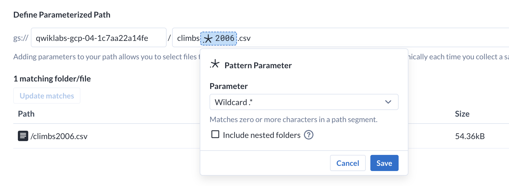
3. Select the portion of the path that you would like to parameterize. Notice that all of the climb data are named as "climbs", followed by the year. Highlight the year (2006) in the path.

4. Once some text is highlighted, you can see options to change the highlighted portion of the path into a parameter. Select the Add Pattern Parameter parameter.

5. Choose Wildcard .* from the Parameter dropdown and click Save.

6. This parameter will match any files that begin with "climbs" and ends with ".csv". On the lower portion of the screen, you can see Dataprep update to reflect any files that match the parameter.

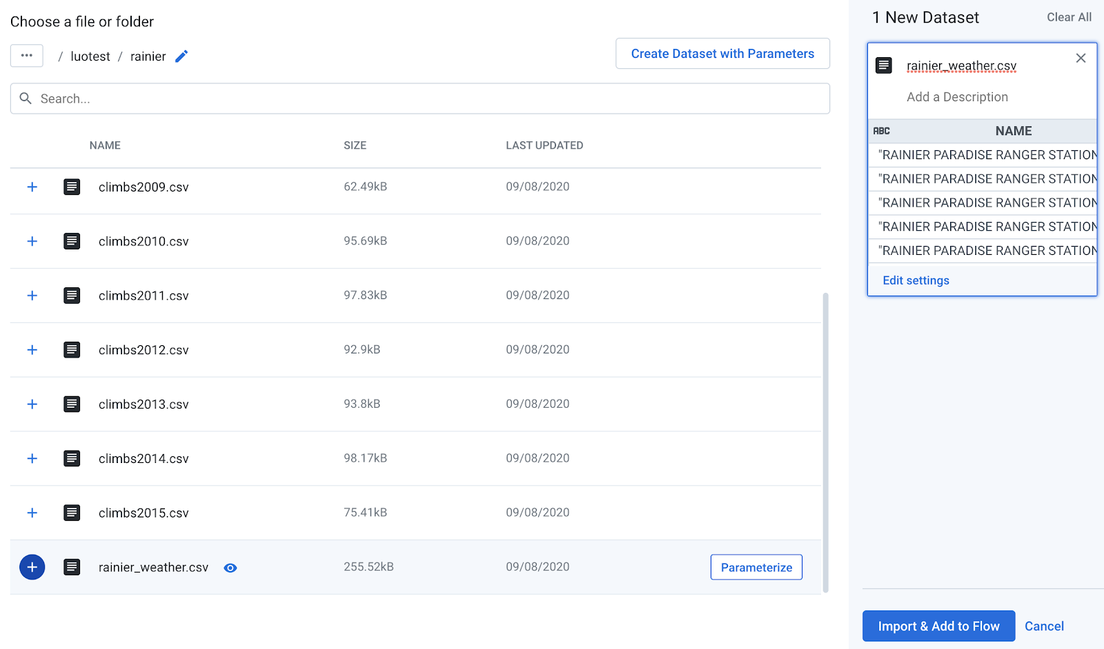
7. Click Create on the bottom right to create a dataset with this parameter. All of the matching files will be concatenated into one large dataset as input for your recipe.

8. Click Import & Add to Flow to add the sources.

A new dataset called Dataset with Parameters is created and placed on the Flow View. A recipe and an output are created automatically for this dataset as well.

Task 3. Take new samples

1. Double click on the recipe node to edit the Dataset with Parameters recipe.

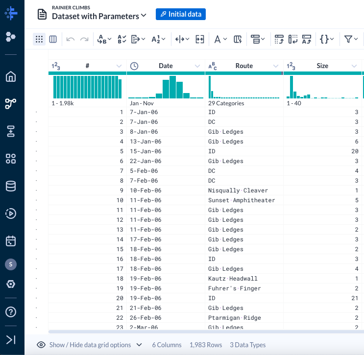
2. When the dataset is first loaded, you may notice the dataset has 6 columns and only 1,983 rows.

3. That row count seems low for a span of 9 years. If you look at the Date column, you may notice in the histogram that it only contains values from 2006. Why is that?

You may also have noticed the notification that showed up in the upper right.

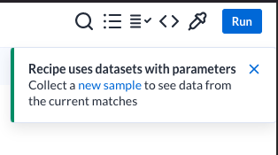
Remember that in Dataprep, you are creating transformations on a sample of the dataset. In this case, it only loaded the first dataset of the parameterized input, just to give you a preview of the data.

4. Click on Initial data box at the top. This will open the Samples Panel.

• Click GOT IT.

Here you can see the current visible samples, as well as other available samples. You can also choose to collect a new sample at any point.

5. Under Collect new sample, select Random.

6. Choose Quick and click Collect to collect a new random sample. A random sample is a sampling technique in which each row has an equal probability of being chosen.

Dataprep is now preparing the new sample for you in the background. The progress can be seen in the panel.

Depending on the size and complexity of the sample, it may take a few minutes to collect. You can continue exploring and manipulating the data with the current sample while the new one collects.

Task 4. Data cleanup

While the sample collects in the background, you can take a brief look at your data. The climb data contains 6 columns:

• # - An incrementing climb ID
• Date - The date of the climb
• Route - The route taken
• Size - The size of the climbing party
• Summit - The number of people who summit the peak
• Leader Zip Code - The zip code of the leader of the climbing party

1. Make a note of the format of the Date column (7-Jan-06).

2. Make a note of the distribution of the Date column. (There are multiple climbing parties per day).

Date manipulation

The standard BigQuery datetime format is yyyy-MM-ddTHH:mm:ss. Since the end goal is to publish this data to BigQuery, it is best to adhere to that format. Dataprep allows for easy manipulation of datetime columns.

1. Click the dropdown next to the Date column and select Format > Change datetime format > Date.

2. This will bring up the Date Format transform builder. Under output format, select the format, in this case, yyyy-MM-dd. Check the preview and then click Add.

Prepare join data

To analyze how the weather affects the summit success rate, the weather data needs to be brought in. That weather data is in another dataset. While Dataprep collects your climb data sample, you can explore the weather dataset.

1. Go back to the Flow view by clicking on the name of the flow RAINIER CLIMBS.

2. At the top right of the Flow View page, click the Add datasets button to add a new dataset to this flow.

3. Click Import datasets on the bottom left of the dialog.

4. Browse back to the same folder on Cloud Storage and add the rainier_weather.csv dataset.
   • Click Import & Add to Flow.

5. A new node appears on the Flow canvas for the weather data. Click the plus (+) sign next to it and select Add new recipe.

6. Rename the Untitled recipe as rainier weather and double click the new recipe node to edit the recipe.

7. The weather data contains the following columns:

   • NAME - The name of the weather station that took the measurements
   • ELEVATION - The elevation of the weather station
   • DATE - The date of forecast
   • Multiday_precipitation_total - The total amount of rainfall across multiple days in inches
   • Multiday_snowfall_total - The total amount of snowfall across multiple days in inches
   • Precipitation_inches - The inches of rainfall for that particular day
   • Snowfall_inches - The inches of snow for that particular day
   • Snow_depth - The depth of snow surrounding the station in inches
   • Temp_max - The forecasted high temperature
   • Temp_min - The forecasted low temperature
   • Temp_observed - The temperature observed at noon
   • Fog - (Boolean) for foggy weather

Note the format of the dates in this dataset: 2/22/06.

8. Take a few moments to scroll through the dataset and familiarize yourself with the overall structure.

Data cleanup

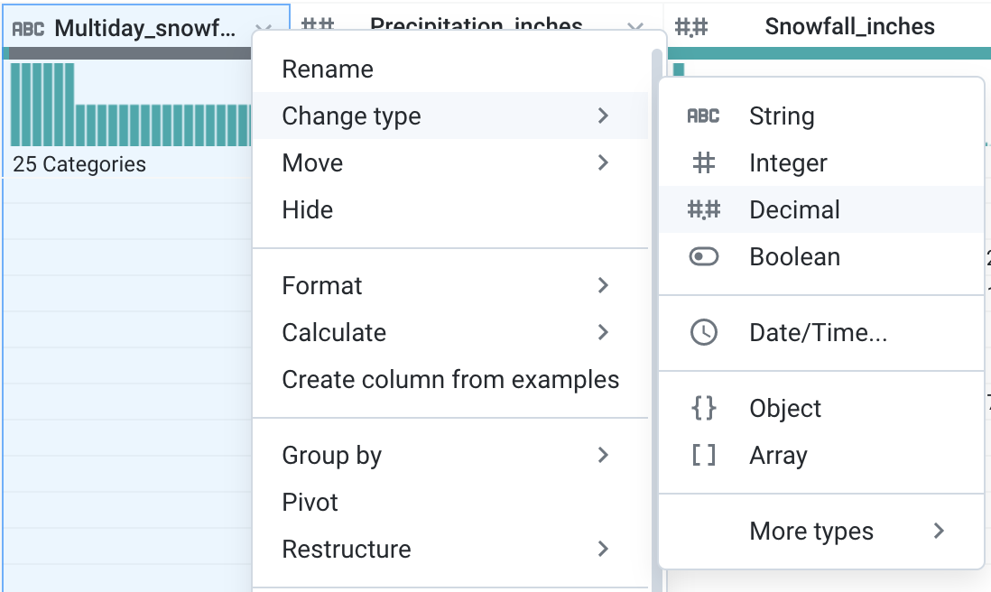
Looking across all of the columns, you can see that Dataprep tried to infer data types based on the most popular values in the columns. However, some of the inferred data types are not what is expected. For example, the majority of values in Snowfall_inches are integers, so the tool inferred the column type as integer, and marked any decimals as mismatched. With dirty data, often you will have to do additional exploration to truly understand what data type is appropriate for each column.

1. For the following columns, change the data type to decimal. Use the dropdown menu next to the column and select Change type > Decimal.

   • Multiday_precipitation_total
   • Multiday_snowfall_total
   • Snowfall_inches

2. Next, take a look at some of the missing values in this dataset. Click on the gray area of the data quality bar for Precipitation_inches. Doing so will cause Dataprep to suggest Transformations for the selected area. Additionally, it highlights the rows that are empty. Scroll through the dataset to see some of the highlighted rows.

3. As you scroll down, you may notice that many of the empty rows in Precipitation_inches have valid values in the Multiday_precipitation_total column.

Not every row follows this pattern, but for the ones that do, it's also very likely that there is a gap in the date as well.

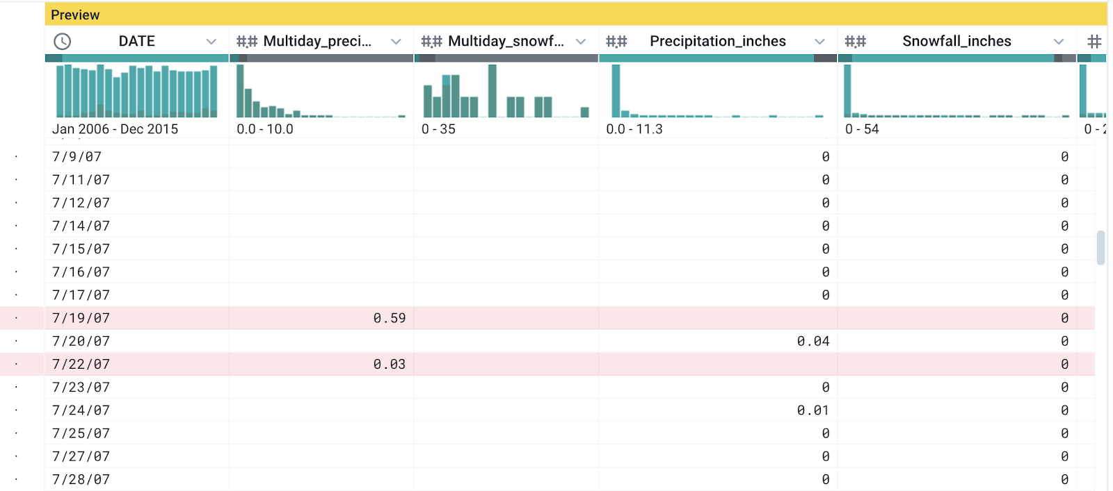
For example, you can see in this screenshot that the data for dates 7/18/07 and 7/21/07 are missing. It seems that for days of constant precipitation, the data is not recorded with daily granularity.

4. It's possible to fill in these dates and values using more complicated logic, but for now, you can coalesce the values in the multi-day and single day precipitation columns to get this dataset in shape to join with the climbs data.

5. Click on the column header of Multiday_precipitation_total to select the column.

6. Hold CTRL or CMD, and click on the header for Precipitation_inches to select 2 columns together.

7. From the suggestions, under Create a new column, choose the COALESCE([Multiday_precipitation_total,Precipitation_inches]) option and Add it.

The COALESCE function returns the first non-empty value found in the 2 columns, essentially merging the columns into a single column.

8. Edit the previous recipe step or add a new recipe step to rename the column to Merged Precipitation.

9. Repeat the Coalesce step for the Snowfall_inches and Multiday_snowfall_total columns. Name the new column Merged Snowfall. Lastly, change the data type from the dropdown menu of the new column to decimal.

Adding comments

While Dataprep displays the transformations in easily readable natural language, if you don't work on a recipe for a long time or share the recipe with others, it may take some deciphering to figure out what the steps do. To help with reusability, you can add comments to your recipes to help annotate and describe your steps.

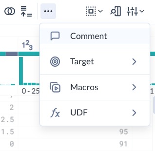
1. Click on the three dots for More actions and click the Comment icon to insert a comment as a new recipe step.

2. Describe the previous steps, ie. "These steps combine the snowfall inches with multi day values".

3. Click Add. Comments will show up in blue with two slashes in front. Comments steps do not change the data and are not executed during job runs.

Moving the Recipe View Line (RVL) and inserting steps

Now that you know how to insert comments, it makes sense to go back and insert a similar comment next to the step that produced the merged precipitation column.

1. To insert a step into the recipe at a specific location, you must change the Recipe View Line (RVL).

The Recipe View Line serves 2 purposes:

• It sets the point at which new steps are added.
• It allows you to view the data at any particular step.

To set the RVL, simply hover in the space in between 2 steps. A gray dotted line will appear to indicate you are mousing over a RVL. Click to set the RVL to that step. The active RVL is indicated by a blue dotted line.

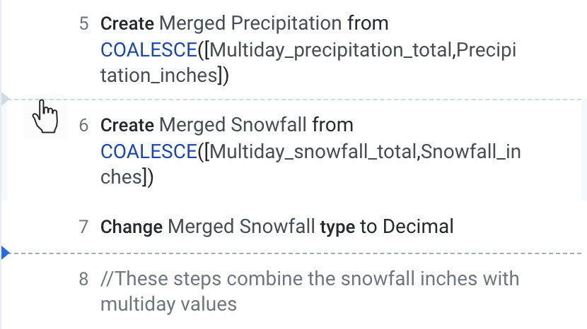
In this screenshot, the RVL is currently between steps 7 and 8.

2. Click between steps 5 and 6 to set the RVL after line 5. When adding the comment, the step will be inserted here.

Notice that, after you have set the RVL after step 5, the column Merged Snowfall no longer shows up in the grid. This is because the steps after the RVL are not displayed in the data grid, allowing you to quickly review the data after different transformations.

Note: You can also set the RVL above step 1 to view the original source data. Note: When you run the job at scale, all recipe steps are still calculated, even the ones beneath the RVL. The RVL only controls what you see in the data grid during design. To prevent steps from being calculated at execution, you have to disable the step.

3. Add the comment "These steps combine the precipitation inches with multi day values" to the recipe.

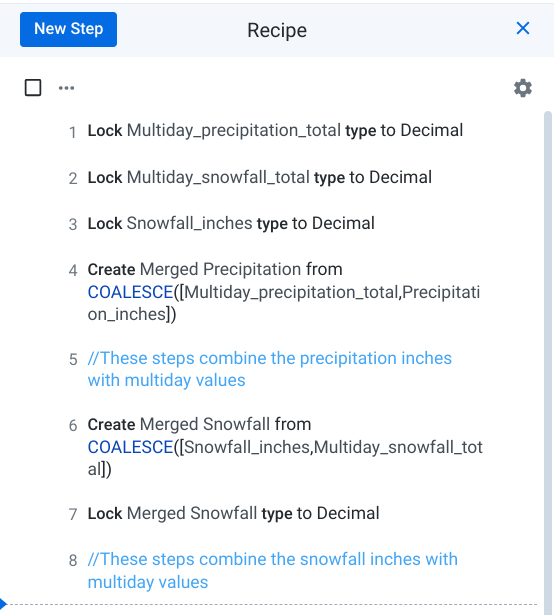
4. Set the RVL back to the bottom of the recipe. Your recipe should now resemble the following:

Aggregate data

By now, your random sample collection on the climb data should be finished.

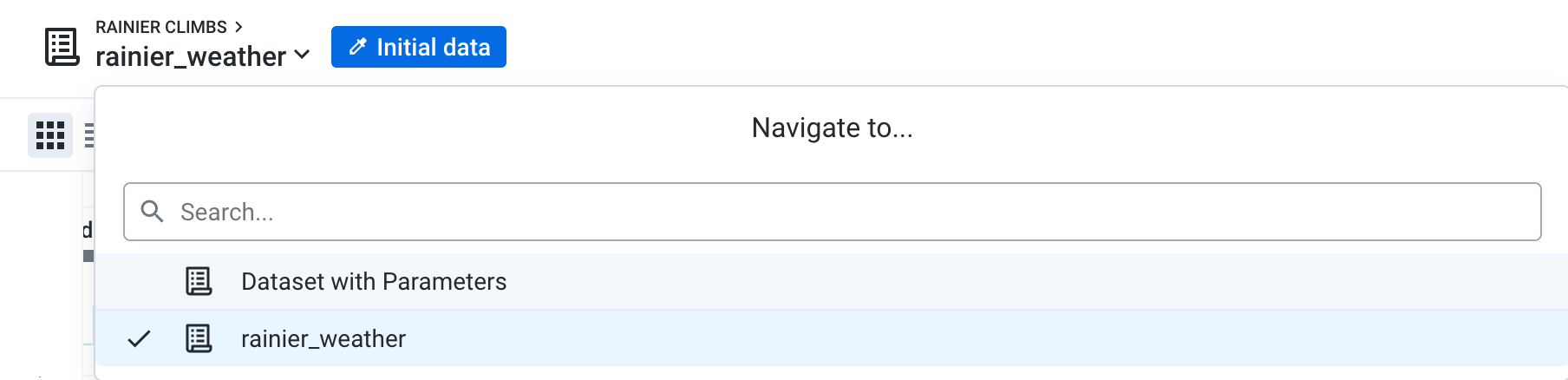
1. Quickly switch to the climb data by clicking on the dropdown next to the recipe name at the top.

2. Click on Dataset with Parameters to quickly switch to the other recipe in the flow.

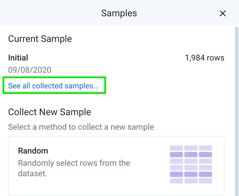
3. Once the recipe is switched, click on Initial data again to open the Samples panel.

4. In the Samples panel, click on See all collected samples.

5. Under Available samples, you should see 2 options: Initial, which is currently selected, and Random. Click on Random to switch to that sample.

6. Click Load. Once the sample is loaded, you should see:

• More rows
• A larger distribution of dates in the Dates column.

Note: Because the rows are randomly selected, the data you see on your screen will deviate from the screenshots in this lab.

Now that you have more rows of data, you can summarize the data to make downstream analysis easier. As you saw when you initially opened this dataset, the climbing dataset has multiple parties per day.

7. Click the Pivot icon to create a pivot table.

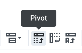
8. A pivot table is a table of statistics that summarizes the data of a more extensive table. Dataprep allows you to build tables with ease by showing you a preview of the resulting table.

In the Row labels section, select the Date column.

Note how the grid changes to show you how the table will look.

9. In the Values section, enter these two: SUM(Size) & SUM(Summit).

The other columns (#* and *Leader Zip Code) will be dropped out as they are not necessary for the analysis.

10. Click Add to accept the aggregation. This pivot summarizes the total number of climbers who set off and summited on each day.

11. You can now calculate the overall success rate for any given day by dividing the sum_Summit by sum_Size. From the toolbar, click the Functions icon then select Math > DIVIDE.

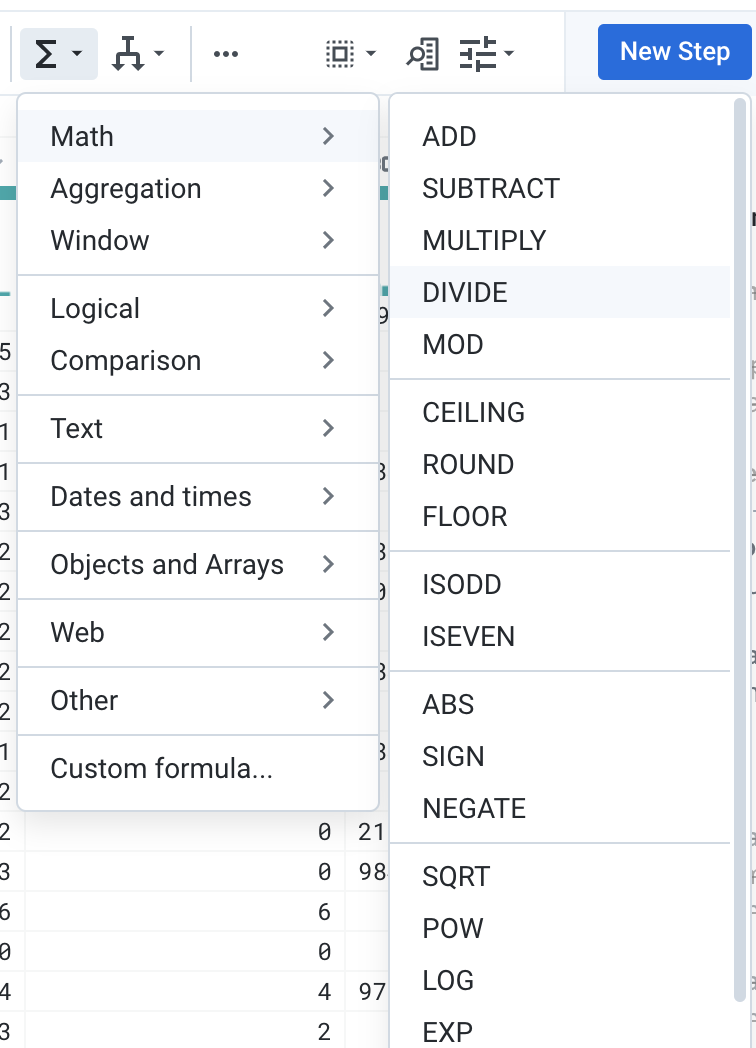
12. For the formula, use DIVIDE(sum_Summit, sum_Size) and name the new column Summit rate. Click Add.

Conditionals and cases

Depending on your sample, you may see that the histogram for the Summit rate shows values above 1.

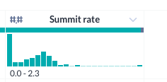
This is odd, because a summit rate above 1 would mean that more people summited than ascended the mountain on a given day. This could indicate that people are camping on the mountain across multiple days or changing expedition groups, but it might skew some of your analysis if the success rate is over 100%. Next, you will create a condition to fix some of the issues.

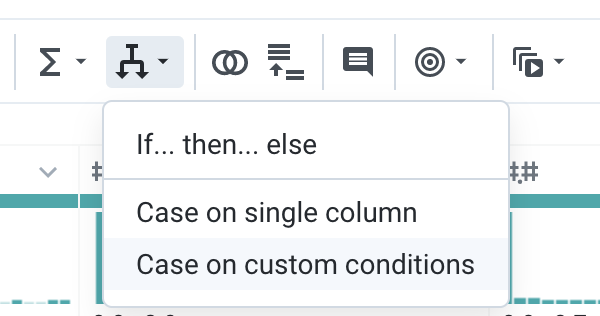
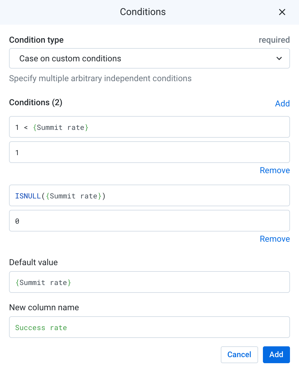
1. From the toolbar, choose Conditions > Case on custom conditions.

2. In the Conditions, the first box is the condition to evaluate and the second box is the value if the case is true. Enter 1 < {Summit rate} into the first box and 1 into the second box. This means, if the summit rate is over 1, then simply set it to 1. (The curly brackets { } around the column name is used to denote any columns with whitespaces)

3. You can add more cases by clicking on Add next to the Conditions argument.

New condition boxes appear. Enter ISNULL({Summit rate}) into the first box and 0 into the second box. For certain rows with sum_Size of 0, the previous calculation for Summit rate would have divided by 0 and produced a null, so just set that to 0.

4. For Default value, enter {Summit rate}. For any rows that do not evaluate true to the previous conditions, it simply fills in the existing value for Summit rate.

5. Name the new column "Success rate" and add the step to the recipe. Click Add. Your condition should resemble the following:

Join datasets

Now that you have the climbing data summarized to the day level, you are ready to join in the weather data.

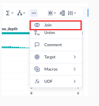
1. Create a new join step by clicking on the three dots for More actions and click the Join icon.

2. Select the weather dataset to join and click Accept.

3. Change the Join type to Left.

4. Edit the Join key to match the Date column = DATE column.

In the preview, notice that Dataprep is able to join on a datetime column that is not in the exact same format.

Also note that because a left join is selected, some rows do not have any matches. (Depending on your sample, the percentage of unmatched rows will vary.)

5. Click Next to select the output columns. Keep the following columns, the rest will be dropped automatically after the join.

   • Date
   • DATE
   • sum_Size
   • sum_Summit
   • Success rate
   • Merged Precipitation
   • Merged Snowfall
   • Snow_depth
   • Temp_observed
   • Fog

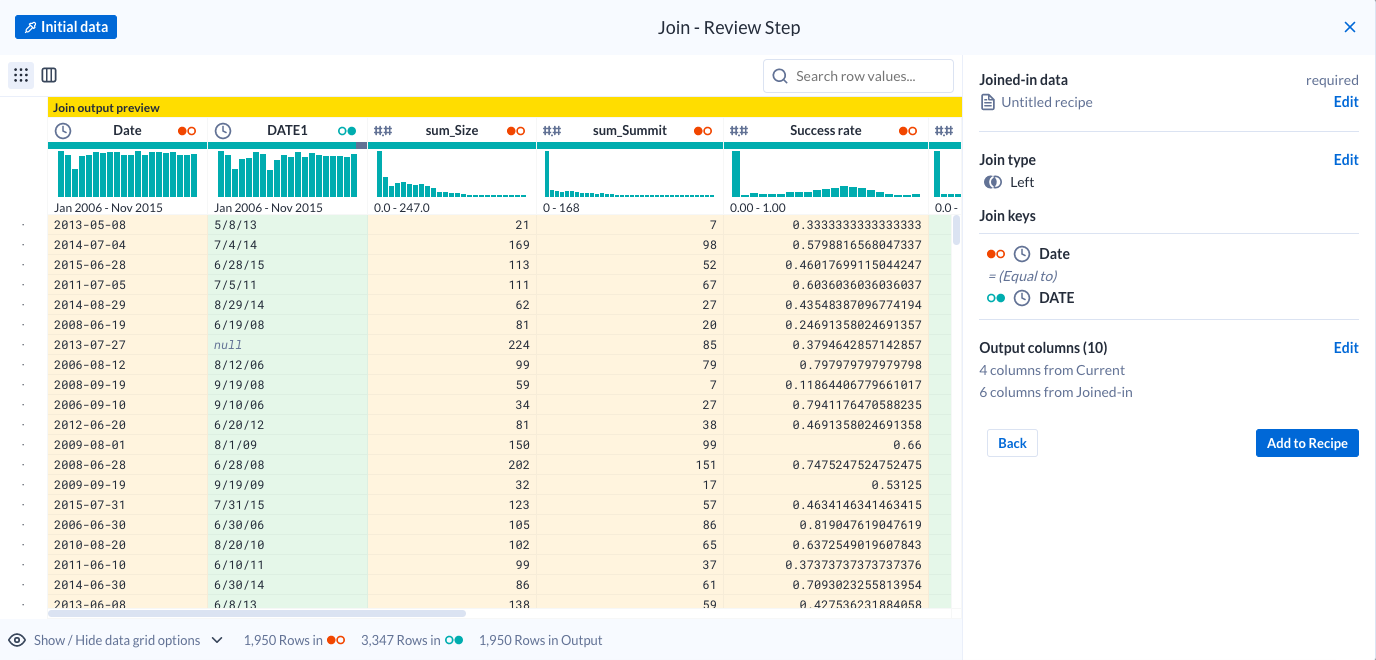
6. Click Review. The join should look something like this:

7. Click Add to recipe.

8. Now that the join is added, you can see that there is weather data missing for some days so you won't be able to use them in your analysis. You can choose to delete the rows where DATE1 is missing or keep them in the dataset.

Task 5. Publish to BigQuery

Now that you have joined the data, you can publish the results to BigQuery.

1. Click the Run button to create an output.

2. In the Publishing Actions section, Dataprep will create a CSV file by default. Hover over the action and click the Edit button to change the publishing destination to BigQuery instead.

3. Choose BigQuery from the list of systems on the left.

4. Choose the Dataprep database and click Create a new table on the right.

5. Based on the column names you created, you should see an error message on the top.

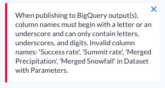
This is indicating that BigQuery cannot take column names with spaces in it and your dataset has a few of these.

6. Click Cancel to exit the Publishing action dialog, and Cancel again to exit the Run Job dialog. Open up the Dataset with Parameter recipe again.

7. Dataprep can quickly fix up issues with column names by removing all special characters. Click on the chevron next to any column and choose Rename.

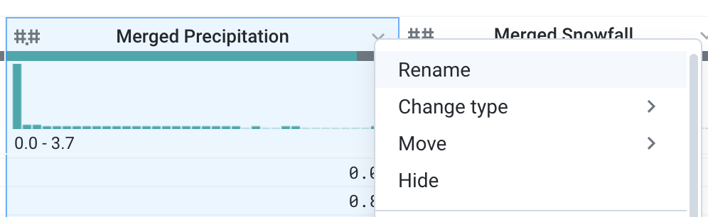
8. By default, the Rename transform will ask you to manually rename the column. However, it also comes with several pre-built functions, including a general cleaning function.

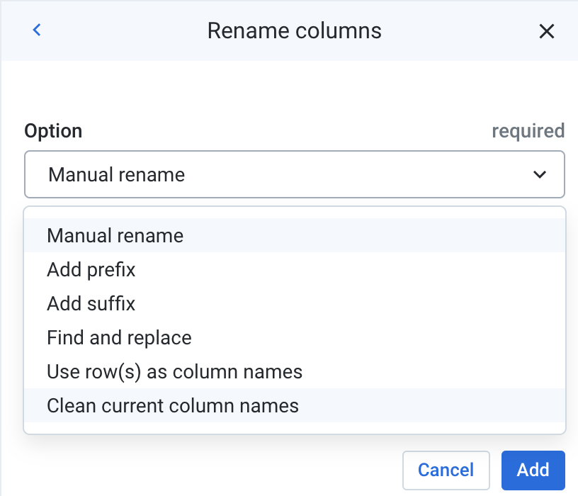
Under the Option dropdown, choose Clean current column names. Notice how the preview affects all columns and has replaced any spaces with underscores. Click Add.

9. Now that the column names are fixed, repeat Steps 1-4 and create a new table called RainierLab. Choose Truncate the table every run and Update the destination.

10. Click Run. This can take several minutes.

Click Check my progress to verify the objective. Publish to BigQuery

Visualize the results

Once the job is finished, build a quick visualization of the data.

1. Return to the Cloud Console and from the Navigation menu select BigQuery. If prompted click Done.

2. In the Query editor, run the following query:

select * from Dataprep.RainierLab;

3. Once the results are returned, click the Explore Data dropdown and select Explore with Looker Studio. This will open Data Studio in another tab.

4. Accept all the agreements for Data Studio.

5. Now you can build a simple visualization. Click Add a chart and choose Line > Stacked Combo chart.

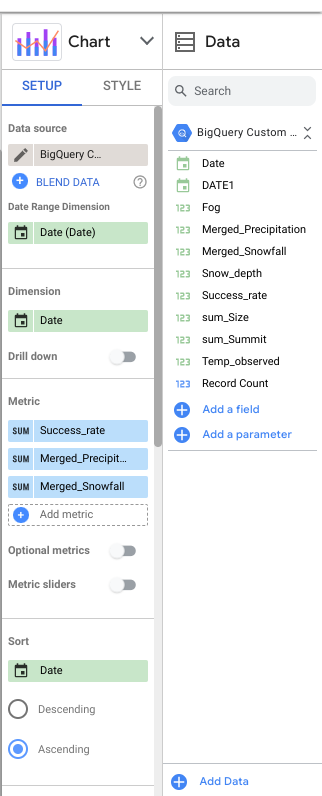
6. In the Setup tab on the right, keep Date Range Dimension as Date (Date) and Dimension as Date.

7. Toggle Optional metrics. Drag Success_rate, Merged_Precipitation, and Merged_Snowfall from the Available Fields to the Metric section. Remove the other metrics and position your Success_rate metric above the others.

8. Lastly, sort by Date ascending. Your configuration should resemble the following:

9. In the Style tab, set the Axis for Series #1 to Right, and the rest of the Series to Left.

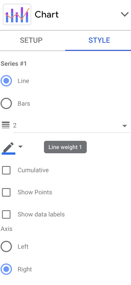
You can play around with the other style settings to whatever suits your taste.

10. Your graph should resemble something like this.

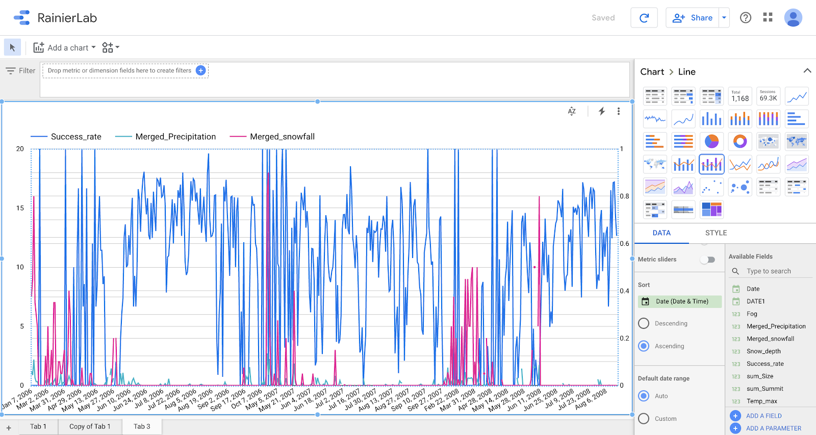
Based on the graph, what can you conclude about the relation of summit success relative to precipitation and snowfall?

11. You can play around with the other features by dragging them from Available Fields into metrics. Is there a better predictor of summit success?

Task 6. Optional - Export your flow

In your own Dataprep project, all of the flows are saved and can be reused. However, for Qwiklabs, these projects are temporary and deleted after the lab. Dataprep allows you to export your flows to use with version control systems, or import them into another environment or share them with colleagues. To save your work for the next lab, you can export the flow you created.

1. Return to the Rainier Climb Flow View.

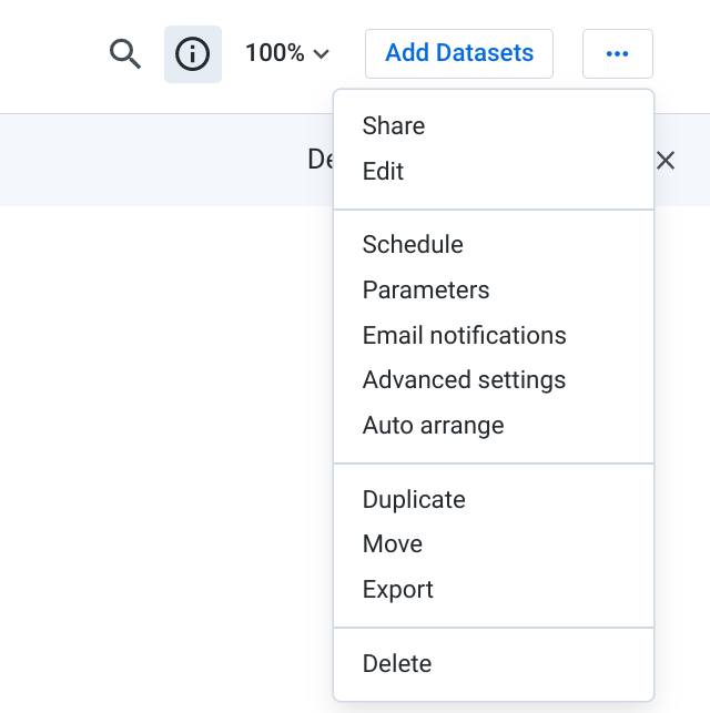
2. On the top right, open the More Menu (...) and select Export.

3. Save the zip file to your local desktop as flow_Rainier_Climbs.zip. You can use this file in the next lab if you so choose.

Congratulations!

In this lab, you got hands-on experience with Dataprep by creating parameterized datasets, leveraging new samples, and creating conditional cases and aggregations. You also manipulated datetimes, cleaned headers to publish to BigQuery, and visualized your results in Data Studio.

Finish your quest

This self-paced lab is part of the Transform and Clean your Data with Dataprep by Alteryx on Google Cloud quest. A quest is a series of related labs that form a learning path. Completing this quest earns you a badge to recognize your achievement. You can make your badge or badges public and link to them in your online resume or social media account. Enroll in this quest and get immediate completion credit. Refer to the Google Cloud Skills Boost catalog for all available quests.

Next steps / Learn more

• Explore Dataprep Professional Edition with a free 30-day trial available. Please make sure to sign out from your temporary Qwiklabs account and re-sign with your Google Cloud valid email. Advanced features, such as additional connectivity, pipeline orchestration, and adaptive data quality are also available in the Premium edition that you can explore in the Google Cloud Marketplace.

• Read the how-to guides to learn how to discover, cleanse, and enhance data with Google Dataprep.

Google Cloud training and certification

...helps you make the most of Google Cloud technologies. Our classes include technical skills and best practices to help you get up to speed quickly and continue your learning journey. We offer fundamental to advanced level training, with on-demand, live, and virtual options to suit your busy schedule. Certifications help you validate and prove your skill and expertise in Google Cloud technologies.

Manual Last Updated January 30, 2024

Lab Last Tested January 30, 2024

Copyright 2024 Google LLC All rights reserved. Google and the Google logo are trademarks of Google LLC. All other company and product names may be trademarks of the respective companies with which they are associated.